pyprocessmacro
Conditional Process Analysis in Python
The Process Macro by Andrew F. Hayes has helped thousands of researchers in their analysis of moderation, mediation, and conditional processes. Unfortunately, Process was only available for proprietary softwares (SAS and SPSS), which means that students and researchers had to purchase a license of those softwares to make use of the Macro.
Because of the growing popularity of Python in the scientific community, I decided to implement the features of the Process Macro into an open-source library, that researchers will be able to use without relying on proprietary softwares. pyprocessmacro is open-source, and released under a MIT license.
1. Features
A. Current Implementation
In the current version, pyprocessmacro replicates the following features from the original Process Macro v2.16:
- All models (1 to 76), with the exception of Model 6 (serial mediation) are supported, and have been numerically tested for accuracy against the output of the original Process macro (see the
test_models_accuracy.py) - Estimation of binary/continuous outcome variables. The binary outcomes are estimated in Logit using the Newton-Raphson convergence algorithm, the continuous variables are estimated using OLS.
- Estimation of (conditional) direct and indirect effects
- Indices for Partial/Conditional/Moderated Moderated Mediation
- Automatic generation of spotlight values for continuous/discrete moderators.
- Rich set of options to tweak the estimation and display of the different models: (almost) all the options from Process exist in pyprocessmacro. See the documentation for more details
B. Changes and Improvements
The following changes and improvements have been made from the original Process Macro:
- Variable names can be of any length, and even include spaces and special characters.
- All mediation models support an infinite number of mediators (versus a maximum of 10 in Process).
- Normal theory tests for the indirect effect(s) are not reported, as the bias-corrected bootstrapping approach is now widely accepted and in most cases more robust.
- Plotting capabilities: pyprocessmacro can generate the plot of direct and indirect effects at various levels of the moderators.
- Fast estimation process: pyprocessmacro leverages the capabilities of NumPy to efficiently compute a large number of bootstrap estimates, which dramatically speeds up the estimation of complex models.
- Transparent bootstrapping: pyprocessmacro automatically store the bootstrap estimates for convenient inspection, and explicitely reports the samples that have been discarded because of numerical instability.
C. Missing Features
In the current version, the following features have not yet been ported to pyprocessmacro:
- Support for categorical independent variables.
- Generation of individual fixed effects for repeated measures.
- R² improvement from moderators in moderation models (1, 2, 3).
- Estimation of serial mediation (Model 6)
- Some options (
normal,varorder, …). pyprocessmacro will issue a warning if you are trying to use an option that has not been implemented.
2. Installation and Usage
A. Installation
You can install pyprocessmacro with pip:
pip install pyprocessmacroor with conda:
conda install pyprocessmacro -c conda-forgeB. Minimal Example
import warnings

import matplotlib.pyplot as plt
import pandas as pd
from pyprocessmacro import Process

warnings.filterwarnings("ignore", category=DeprecationWarning)

df = pd.read_csv("data.csv")
p = Process(data=df, model=4, x="Effort", y="Success", m=["MediationSkills"])
p.summary()
Process successfully initialized.
Based on the Process Macro by Andrew F. Hayes, Ph.D. (www.afhayes.com)
****************************** SPECIFICATION ****************************
Model = 4
Variables:
Cons = Cons
x = Effort
y = Success
m1 = MediationSkills
Sample size:
1000
Bootstrapping information for indirect effects:
Final number of bootstrap samples: 5000
Number of samples discarded due to convergence issues: 0
***************************** OUTCOME MODELS ****************************
Outcome = Success
OLS Regression Summary
R² Adj. R² MSE F df1 df2 p-value
0.9699 0.9698 2.0003 16083.2644 2 997 0.0000
Coefficients
coeff se t p LLCI ULCI
Cons 1.8755 0.0664 28.2317 0.0000 1.7453 2.0057
Effort 0.0653 0.0500 1.3060 0.1919 -0.0327 0.1632
MediationSkills 1.0053 0.0066 153.1107 0.0000 0.9925 1.0182
-------------------------------------------------------------------------
Outcome = MediationSkills
OLS Regression Summary
R² Adj. R² MSE F df1 df2 p-value
0.2648 0.2633 46.4881 359.3661 1 998 0.0000
Coefficients
coeff se t p LLCI ULCI
Cons 4.1472 0.2921 14.1967 0.0000 3.5746 4.7197
Effort 3.9167 0.2066 18.9570 0.0000 3.5118 4.3216
-------------------------------------------------------------------------
********************** DIRECT AND INDIRECT EFFECTS **********************
Direct effect of Effort on Success:
Effect SE t p LLCI ULCI
0.0653 0.0500 1.3060 0.1919 -0.0327 0.1632
Indirect effect of Effort on Success:
Effect Boot SE BootLLCI BootULCI
MediationSkills 3.9377 0.2362 3.4967 4.4323Two important notes: * There is no argument varlist in pyprocessmacro: this list is automatically inferred from the variable names given to x, y, m, etc… * The argument supplied to m is a list, even if you have a single mediator.
Other than this, the syntax for pyprocessmacro is (almost) identical to that of Process. Unless this documentation mentions otherwise, you can assume that all the options/keywords from Process exist in pyprocessmacro.
Once the object is initialized, its summary() method is used to display the estimation results.
C. Suppress the Initialization Message
When the Process object is initialized by Python, it displays various information about the model (model number, list of variables, sample size, number of bootstrap samples, etc…). If you wish not to display this information, just add the argument suppr_init=True when initializing the model.
p = Process(
    data=df,
    model=4,
    x="Effort",
    y="Success",
    m=["MediationSkills"],
    controls=["ModerationSkills"],
    controls_in="all",
    suppr_init=True,
)
D. Adding Statistical Controls
In Process, the controls are defined as “any argument in the varlist that is not the IV, the DV, a moderator, or a mediator.”
In pyprocessmacro, the list of variables to include as controls have to be explicitely specified in the “controls” argument.
p = Process(
    data=df,
    model=4,
    x="Effort",
    y="Success",
    m=["MediationSkills"],
    controls=["ModerationSkills"],
    controls_in="all",
    suppr_init=True,
)
The equation(s) to which the controls are added is specified through a controls_in argument:
x_to_mmeans that the controls will only be added in the path from the IV to the mediator(s) only.all_to_ymeans that the controls will only be added in the path from the IV and the mediators to the DV.allmeans that the controls will be added in all equations.
E. Logistic Regressions for Binary Outcomes
The original Process Macro automatically uses a Logistic (instead of OLS) regression when it detects a binary outcome.
pyprocessmacro favors a more explicit approach, and requires you to set the parameter logit to True if your DV should be estimated using a Logistic regression. It goes without saying that this will return an error if your DV is not dichotomous.
p = Process(
    data=df,
    model=4,
    x="Effort",
    y="SuccessBinary",
    m=["MediationSkills"],
    controls=["ModerationSkills"],
    logit=True,
    suppr_init=True,
)
F. Spotlight Values for Moderators
In Process as in pyprocessmacro, the spotlight values of the moderators are defined as follow:
- By default, the spotlight values are equal to M - 1SD, M and M + 1SD, where M and SD are the mean and standard deviation of that variable.
- If the option
quantile=Trueis specified, then the spotlight values for each moderator are the 10th, 25th, 50th, 75th and 90th percentile of that variable. - If a moderator is a discrete variable, the spotlight values are those discrete values.
In Process, custom spotlight values can be applied to each moderator q, v, z, … through the arguments qmodval, vmodval, zmodval…
In pyprocessmacro, the user must instead supply custom values for each moderator in a dictionary passed to the modval parameter:
p = Process(
    data=df,
    model=13,
    x="Effort",
    y="Success",
    w="Motivation",
    z="SkillRelevance",
    m=["MediationSkills"],
    modval={
        "Motivation": [-5, 0, 5],
        # Moderator 'Motivation' at values -5, 0 and 5
        "SkillRelevance": [-1, 1]
        # Moderator 'SkillRelevance' at values -1 and 1
    },
    suppr_init=True,
)
3. Accessing the Results
A. summary()
This method replicates the output that you would see in Process, and displays the following information:
- Model summaries and parameters estimates for all outcomes (i.e. the independent variable, and the mediator(s)).
- If the model has a moderation, conditional effects at the spotlight values of the moderator(s).
- If the model has a mediation, direct and indirect effects.
- If the model has a moderation and a mediation, conditional direct and indirect effects at values of the moderator(s).
- If those statistics are relevant, indices for partial, conditional, and moderated moderated mediation will be reported.
p = Process(
    data=df, model=4, x="Effort", y="Success", m=["MediationSkills"], suppr_init=True
)
p.summary()
***************************** OUTCOME MODELS ****************************
Outcome = Success
OLS Regression Summary
R² Adj. R² MSE F df1 df2 p-value
0.9699 0.9698 2.0003 16083.2644 2 997 0.0000
Coefficients
coeff se t p LLCI ULCI
Cons 1.8755 0.0664 28.2317 0.0000 1.7453 2.0057
Effort 0.0653 0.0500 1.3060 0.1919 -0.0327 0.1632
MediationSkills 1.0053 0.0066 153.1107 0.0000 0.9925 1.0182
-------------------------------------------------------------------------
Outcome = MediationSkills
OLS Regression Summary
R² Adj. R² MSE F df1 df2 p-value
0.2648 0.2633 46.4881 359.3661 1 998 0.0000
Coefficients
coeff se t p LLCI ULCI
Cons 4.1472 0.2921 14.1967 0.0000 3.5746 4.7197
Effort 3.9167 0.2066 18.9570 0.0000 3.5118 4.3216
-------------------------------------------------------------------------
********************** DIRECT AND INDIRECT EFFECTS **********************
Direct effect of Effort on Success:
Effect SE t p LLCI ULCI
0.0653 0.0500 1.3060 0.1919 -0.0327 0.1632
Indirect effect of Effort on Success:
Effect Boot SE BootLLCI BootULCI
MediationSkills 3.9377 0.2362 3.4967 4.4323B. outcome_models
This command gives you individual access to each of the outcome models through a dictionary. This allows you to recover the model and parameters estimates for each outcome.
Each OutcomeModel object has the following methods:
summary()prints the full summary of the model (as Process does).model_summary()returns a DataFrame of goodness-of-fit statistics for the model.coeff_summary()returns a DataFrame of estimate, standard error, corresponding z/t, p-value, and confidence interval for each of the parameters in the model.estimation_resultsgives you access to a dictionary containing all the statistical information of the model.
# The model for the outcome "MediationSkills"
model_medskills = p.outcome_models["MediationSkills"]

# Print the summary for this model
print(model_medskills.summary())
Outcome = MediationSkills
OLS Regression Summary
R² Adj. R² MSE F df1 df2 p-value
0.2648 0.2633 46.4881 359.3661 1 998 0.0000
Coefficients
coeff se t p LLCI ULCI
Cons 4.1472 0.2921 14.1967 0.0000 3.5746 4.7197
Effort 3.9167 0.2066 18.9570 0.0000 3.5118 4.3216# Acccess the DataFrame of estimates
model_medskills.coeff_summary()| coeff | se | t | p | LLCI | ULCI | |
|---|---|---|---|---|---|---|
| Cons | 4.147182 | 0.292122 | 14.196744 | 8.392403e-42 | 3.574633 | 4.719730 |
| Effort | 3.916699 | 0.206610 | 18.956953 | 1.096456e-68 | 3.511751 | 4.321648 |
# Access the R² of the model
model_medskills.estimation_results["R2"]0.2647525050214643Note that the methods are called from the model_medskills object! If you call p.coeff_summary(), you will get an error.
C. direct_model
When the Process model includes a mediation, the direct effect model can be accessed. It implements the following methods: * summary() prints the full summary of the direct effects, as printed when calling Process.summary(). * coeff_summary() returns a DataFrame of estimate, standard error, t-value, p-value, and confidence interval for each of the (conditional) direct effect(s).
direct_effect_model = p.direct_model

# Store the DataFrame of estimates into a variable.
df_params_direct = direct_effect_model.coeff_summary()

# Print the summary for this model
print(direct_effect_model.summary())
Direct effect of Effort on Success:
Effect SE t p LLCI ULCI
0.0653 0.0500 1.3060 0.1919 -0.0327 0.1632Note that the methods are called from the direct_effect_model object! If you call p.coeff_summary(), you will get an error.
D. indirect_model
When the Process model includes a parallel mediation, the indirect effect model can be accessed as well. It implements the following methods:
summary()prints the full summary of the indirect effects, and other related indices, as printed by Process.summary().coeff_summary()returns a DataFrame of indirect effect(s) and their SE/CI for each of the mediation pathsMM_index_summary()returns a DataFrame of indices for Moderated Mediation, and their SE/CI, for each of the mediation paths. If the model does not compute a MM, this will return an error.PMM_index_summary()returns a DataFrame of indices for Partial Moderated Mediation, and their SE/CI, for each of the moderators and mediation paths. If the model does not compute a PMM, this will return an error.CMM_index_summary()returns a DataFrame of indices for Conditional Moderated Mediation, and their SE/CI, for each of the moderators and mediation paths. If the model does not compute a CMM, this will return an error.MMM_index_summary()returns a DataFrame of indices for Moderated Moderated Mediation, and their SE/CI, for each of the mediation paths. If the model does not compute a MMM, this will return an error.
# The model for the direct effect
indirect_effect_model = p.indirect_model

# Store the DataFrame of estimates into a variable.
df_params_direct = indirect_effect_model.coeff_summary()
Note that the methods are called from the indirect_effect_model object! If you call p.coeff_summary(), you will get an error.
4. Recover the Bootstrap Estimates
The original Process macro allows you to save the parameter estimates for each bootstrap sample by specifying the save keyword. The Macro then returns a new dataset of bootstrap estimates.
In pyprocessmacro, this is done by calling the method get_bootstrap_estimates(), which returns a DataFrame containing the parameters estimates. Each row represents a bootstrap repetition, and the columns are explicitely labeled to identity the variables and the model.
boot_estimates = p.get_bootstrap_estimates()  # Called from the Process object directly.
boot_estimates.groupby("OutcomeName").head(
    5
) # Estimates in the first 5 bootstrap samples| BootSample | OutcomeName | Cons | Effort | MediationSkills | |
|---|---|---|---|---|---|
| 0 | 0 | Success | 1.891449 | 0.019013 | 1.010788 |
| 1 | 1 | Success | 1.999370 | 0.047046 | 0.991365 |
| 2 | 2 | Success | 1.879890 | -0.013556 | 1.017109 |
| 3 | 3 | Success | 1.889204 | 0.018213 | 1.007163 |
| 4 | 4 | Success | 1.781783 | 0.085147 | 1.010819 |
| 5000 | 0 | MediationSkills | 4.008258 | 4.035267 | NaN |
| 5001 | 1 | MediationSkills | 4.097921 | 3.992029 | NaN |
| 5002 | 2 | MediationSkills | 3.842924 | 3.913002 | NaN |
| 5003 | 3 | MediationSkills | 4.206325 | 3.959671 | NaN |
| 5004 | 4 | MediationSkills | 4.140622 | 3.867696 | NaN |
5. Spotlight and Floodlight Analysis
pyprocessmacro offers four convenience functions for spotlight and floodlight analysis: * floodlight_direct_effect() runs a floodlight analysis on the direct effect * floodlight_indirect_effect() runs a floodlight analysis on the indirect effect * spotlight_direct_effect() runs a spotlight analysis on the direct effect * spotlight_indirect_effect() runs a spotlight analysis on the indirect effect
Let’s consider a new model, in which the direct and indirect paths are moderated by two moderators (Process Model 12).
df = pd.read_csv("data.csv")
p = Process(
    data=df,
    model=12,
    x="Effort",
    y="Success",
    w="Motivation",
    z="SkillRelevance",
    m=["MediationSkills", "ModerationSkills"],
    suppr_init=True,
)
A. Spotlight Analysis
The two functions spotlight_direct_effect() and spotlight_indirect_effect() return the conditional direct/indirect effects at various levels of the moderator(s).
spotlight_direct_effect() can be called without any argument, but spotlight_indirect_effect() requires you to specify the name of the mediator for which you want to compute the indirect effects,
By default, the spotlight values are the ones provided at initialization, but you can change them through the spotval argument:
p.spotlight_indirect_effect("MediationSkills", spotval={"SkillRelevance": [0, 1]})| Effect | Boot SE | LLCI | ULCI | Motivation | SkillRelevance | |
|---|---|---|---|---|---|---|
| 0 | 0.946619 | 0.070250 | 0.802410 | 1.083349 | 0.012446 | 0.0 |
| 1 | 1.958880 | 0.077158 | 1.809195 | 2.114763 | 0.012446 | 1.0 |
| 2 | 1.935696 | 0.078388 | 1.781905 | 2.090382 | 1.013064 | 0.0 |
| 3 | 3.939386 | 0.134884 | 3.681146 | 4.214726 | 1.013064 | 1.0 |
| 4 | 2.924774 | 0.116568 | 2.696748 | 3.152203 | 2.013683 | 0.0 |
| 5 | 5.919893 | 0.202711 | 5.527697 | 6.328969 | 2.013683 | 1.0 |
B. Floodlight Analysis
floodlight_direct_effect() and floodlight_indirect_effect() use an iteration procedure to find the Johnson-Neyman region(s) of significance for the direct/indirect effect.
You must specify: * The name of the moderator on which to run the Johnson-Neyman procedure * The name of the mediation path (only for floodlight_indirect_effect())
If there are multiple moderators, the analysis is run assuming that all the other moderators are at 0. You can change this behavior through the other_modval argument.
jn_region = p.floodlight_indirect_effect(
    "MediationSkills", "SkillRelevance", other_modval={"Motivation": 1}
)
print(jn_region)
********************** FLOODLIGHT ANALYSIS OF THE INDIRECT EFFECT **********************
----------------------------------- Analysis Details -----------------------------------
Mediator:
MediationSkills
Focal Moderator:
SkillRelevance, Range = [-2.108, 4.502]
Spotlight value for other moderators:
Motivation = 1
----------------------------------- Analysis Results -----------------------------------
The indirect effect is significantly negative on the interval [-2.108, -1.042]
The indirect effect is significantly positive on the interval [-0.8986, 4.502]
****************************************************************************************6. Plotting Capabilities
pyprocessmacro allows you to plot the conditional direct and indirect effect(s), at different values of the moderators.
The methods plot_conditional_indirect_effects() and plot_direct_effects() are identical in syntax, with one small exception: you must specify the name of the mediator for plot_indirect_effects as a first argument.
They return a seaborn.FacetGrid object that can be used to further tweak the appearance of the plot.
A. Basic Usage
When plotting conditional direct (and indirect) effects, the effect is always represented on the y-axis. The various spotlight values of the moderator(s) can be represented on several dimensions:
- On the x-axis (moderator passed to
x). - As a color-code, in which case several lines are displayed on the same plot (moderator passed to
hue). - On different plots, displayed side-by-side (moderator passed to
col). - On different plots, displayed one below the other (moderator passed to
row)
At the minimum, the x argument is required, while the hue, col and row are optional. The examples below are showing what the plots could look like for a model with two moderators.
# Conditional direct effects of Effort, at values of Motivation (x-axis)
g = p.plot_conditional_direct_effects(x="Motivation", hue="SkillRelevance")

# Display figure
g.add_legend(title="")
fig = plt.gcf()
plt.close()
display(fig, metadata=dict(filename="Fig1"))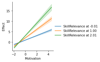
B. Different Spotlight Values
By default, the spotlight values used to plot the effects are the same as the ones passed when initializing Process.
However, you can pass custom values for some, or all, the moderators through the mods_at argument. The library will automatically compute the conditional effects at those new spotlight values, and plot them.
g = p.plot_conditional_indirect_effects(
    med_name="MediationSkills",
    x="Motivation",
    hue="SkillRelevance",
    # Change the spotlight values for SkillRelevance
    modval={"SkillRelevance": [-5, 5]},
)

# Display figure
g.add_legend(title="")
fig = plt.gcf()
plt.close()
display(fig, metadata=dict(filename="Fig2"))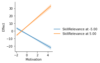
C. Different Visualizations of Uncertainty
The display of confidence intervals for the direct/indirect effects can be customized through the errstyle argument: * errstyle="band" (default) plots a continuous error band between the lower and higher confidence interval. This representation works well when the moderator displayed on the x-axis is continuous (e.g. age), as it allows you to visualize the error at all levels of the moderator. * errstyle="ci" plots an error bar at each value of the moderator on x-axis. It works well when the moderator displayed on the x-axis is dichotomous or has few values (e.g. gender), as it reduces clutter. * errstyle="none" does not show the error on the plot.
g = p.plot_conditional_indirect_effects(
    med_name="MediationSkills",
    x="Motivation",
    hue="SkillRelevance",
    # Dichotomous values for moderators...
    modval={"SkillRelevance": [0, 1], "Motivation": [0, 1]},
    # Call for error bars rather than error bands
    errstyle="ci",
)

# Display figure
g.add_legend(title="")
fig = plt.gcf()
plt.close()
display(fig, metadata=dict(filename="Fig3"))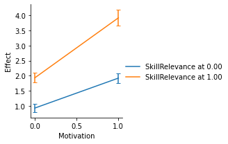
D. Customizing Plots
Under the hood, the plotting functions relies on a seaborn.FacetGrid object, on which the following functions are called:
plt.plotwhenerrstyle="none"plt.plotandplt.fill_betweenwhenerrstyle="band"plt.plotandplt.errorbarwhenerrstyle="ci"
You can pass custom arguments to each of those objects to customize the appearance of the plot:
# Plot: Make the lines bolder
plot_kws = {"lw": 3}
# Errors: Make the CI bolder, red, and remove the 'caps'
err_kws = {"ecolor": "red", "elinewidth": 3, "capsize": 0}
# Grid: Change the aspect ratio of the plot
facet_kws = {"aspect": 2}

g = p.plot_conditional_indirect_effects(
    med_name="MediationSkills",
    x="Motivation",
    errstyle="ci",
    hue="SkillRelevance",
    modval={"Motivation": [-2, -1, 0, 1, 2]},
    plot_kws=plot_kws,
    err_kws=err_kws,
    facet_kws=facet_kws,
)

# Display figure
g.add_legend(title="")
fig = plt.gcf()
plt.close()
display(fig, metadata=dict(filename="Fig4"))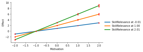
7. About
pyprocessmacro was developed by Quentin André during his Ph.D. in Marketing at INSEAD, France.
His work on this library was made possible by Andrew F. Hayes’ book, by the financial support of INSEAD and by the ADLPartner Ph.D. award.
8. Copyright Notice
The original Process Macro for SAS and SPSS, and its associated files, are copyrighted by Andrew F. Hayes.
The original code must not be edited or modified, and must not be distributed outside of http://www.processmacro.org.
Because pyprocessmacro is a complete reimplementation of the Process Macro, and was not based on the original code, pyprocessmacro is released under a MIT license.
Andrew F. Hayes does not endorse pyprocessmacro: All potential errors, bugs and inaccuracies are my own, and Andrew F. Hayes was not involved in writing, reviewing, or debugging the code.